A step by step manual for using our muscle segmentation
How to use the muscle segmentation framwork
This page provides a comprehensive guide to the functions available in the SegmentationTools package, which is a part of the QMRITools library. The package is designed to assist in the segmentation of medical images, particularly muscles and bones. The tools include functionalities for preparing and visualizing data, defining and configuring various UNET architectures, and training neural networks for segmentation tasks.
The SegmentationTools package offers a range of functions that are organized into key categories:
- Data Visualization: (Placeholder for functions related to visualizing data).
- Data Preparation: Functions for processing and preparing data for segmentation tasks.
- UNet Configuration: Detailed tools for defining, configuring, and managing UNET architectures, including blocks and scaling features.
- Training Networks: Capabilities for training neural networks from scratch or continuing training from existing models.
- Using Networks: How to deploy the trained networks in the current framwork.
General Infromation
Each function is documented with its purpose, input parameters, and expected output, providing a clear understanding of how to use these tools effectively in your segmentation projects. Within QMTITools masks are considered to be binary voluems only containing 0 and 1. Segmentations are considered to be multiple masks all with there own integer label. To work with segmentations various functions have been implemented that can split into masks and the labels, exctract specific labels, replace labels with other values combine segmentations and many more.
SplitSegmentationssplits the segmentation into masks and label numbers.MergeSegmentationsmerges masks into a segmentation. If no labels are provided they are automatically numbered.GetSegmentationLabelsextracts the labels that are present in the segemntation.SelectSegmentationsselects only the segmentions of the given labels.ReplaceSegmentationsreplaces segmentation labels with other label.SmoothSegmentationsmooths each of the individual segmentations using theSmoothMaskfucntion.
For manually drawing ITKSnap is used. Therefore QMRITools has various default ITKSnap label files with stadardized naming, numbering and coloring. These files can be found in the instalation folder of QMRITools in the folder “NeuralNetworks” and are also used for the naming and numbering in the segmentation framework.
- Bones_leg.txt - all bones of the leg (no left or right).
- Muscles_leg_hip.txt - all hip muscles (no left or right).
- Muscles_leg_upper.txt - all upper leg muscles (no left or right).
- Muscles_leg_lower.txt - all lower leg muscles (no left or right).
- Muscles_leg_all.txt - all lower and upper leg muscles and bones (no left or right).
- Muscles_leg.txt - all lower and uppler leg and hip muscles and bones (left and right separate).
1. Data Visualization
To evaluate input or output data for training segmentation networks you want to be able to see and check the data. Therefore QMRITools comprisese several usefull visualization tools for displaying the data. The main visualization function is PlotData which provides a data viewer with various options. However for 3D segmentations the framework also contains a dedicated function for 3D visualsions which is called ‘PlotSegmentations’.
PlotSegmentations[muscleSegmentation, boneSegmentation, voxelsize]
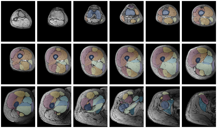
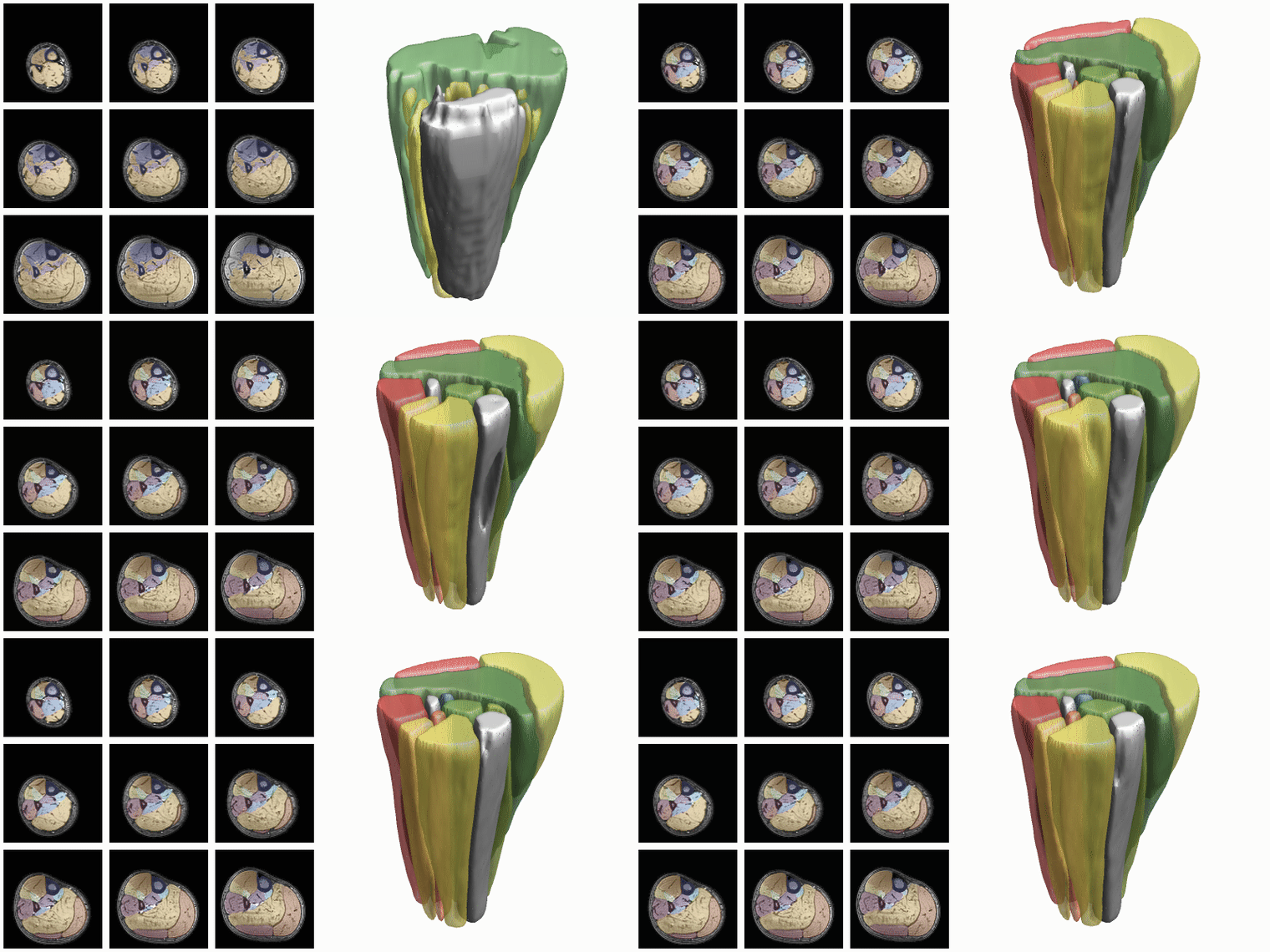
Another way to quickly evaluate the segmenations is using the ‘MakeChannelClassGrid’ which is also used to monitor network training. It takes a training data set with the correspoining labe and makes a image grid of the segmentations.
MakeChannelClassGrid[{data}, seg, {6, 3}]
2. Data preparation
When training networks one of the most important aspects is the quality of training data. Altough humans are, after some training, exelent in manually segmenting muscles thay make mistaces and the slice tot slice vartions can be apparent if one does not use semiautomated methods. Therefore the framework has functions for manipulating, smoothing and evaluating segmentations.
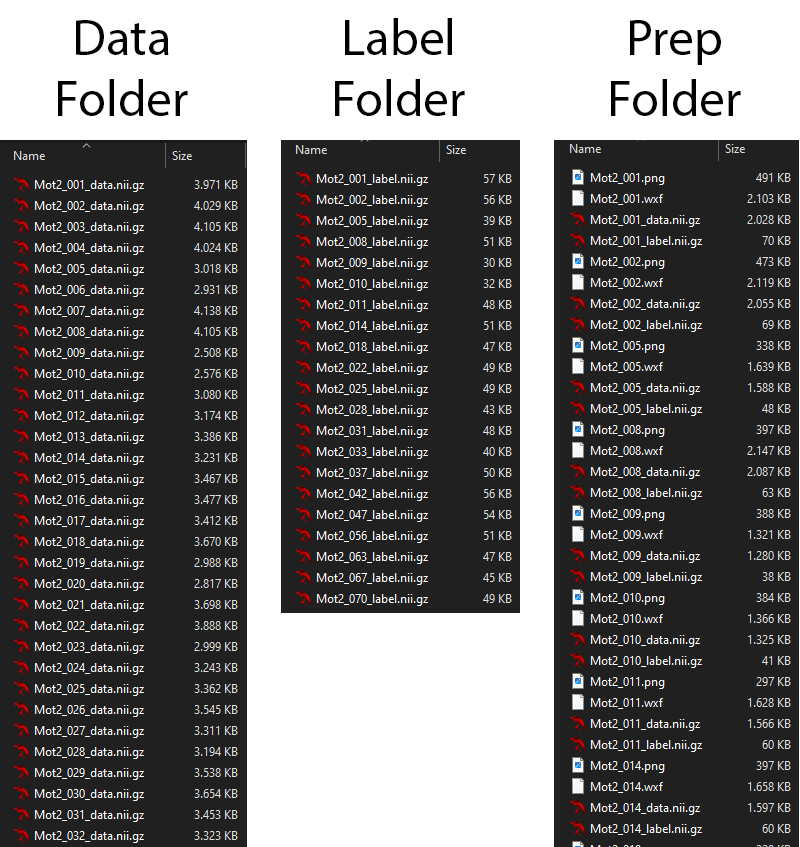
To train the network the data needs to be prepared and stored in a specific format in the training folder. For this the function PrepareTrainingData is used which checks the data qualtiy and can also cleanup the segmentations if needed.
PrepareTrainingData[{segmentaionFolder, dataFolder}, outputFolder,
  TestRun -> True, CleanUpSegmentations -> False,
  LabelTag -> "label", DataTag -> "data"]
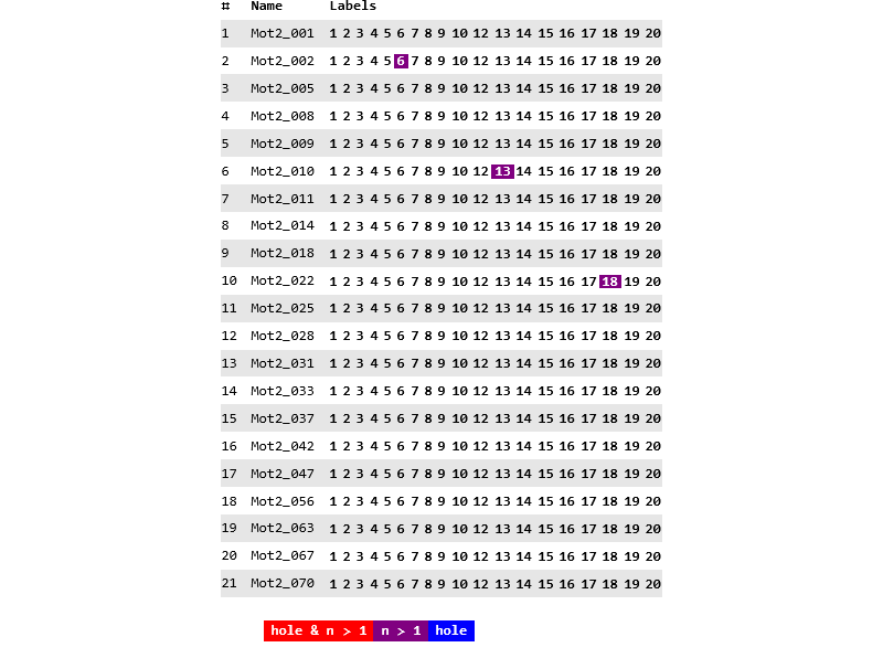
In the example below there are 21 datasets identified which all have 20 labels (excluding the backgroud) of which a few segementaions that are not 1 continuous volume.
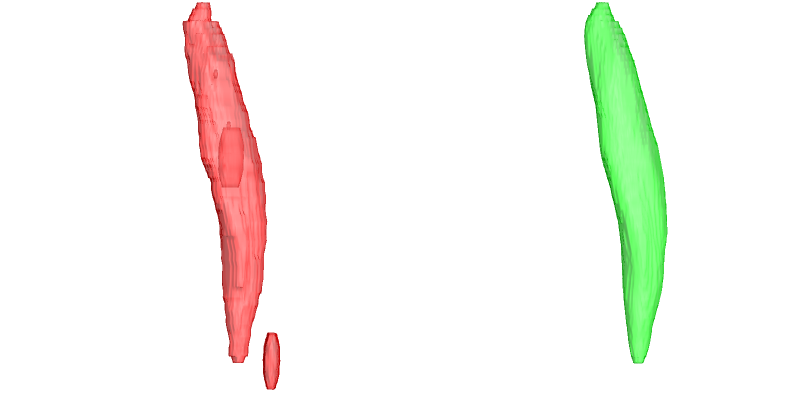
When segmentations contain mistaces or inperfections there are multiple functions that can help, where the most advanced and complete is SmoothSegmentation which allows to remove holes, select the number of segmentation components and allows for itterative surface smooting. This is shown in the example below where the original segmentation has a hole, and additional volume and has a rough surface.
segOut = SmoothSegmentation[segIn, MaskComponents -> 1,
  MaskClosing -> True, MaskDilation -> 0,
  MaskFiltKernel -> 2, SmoothItterations -> 3];
3. UNet Configuration
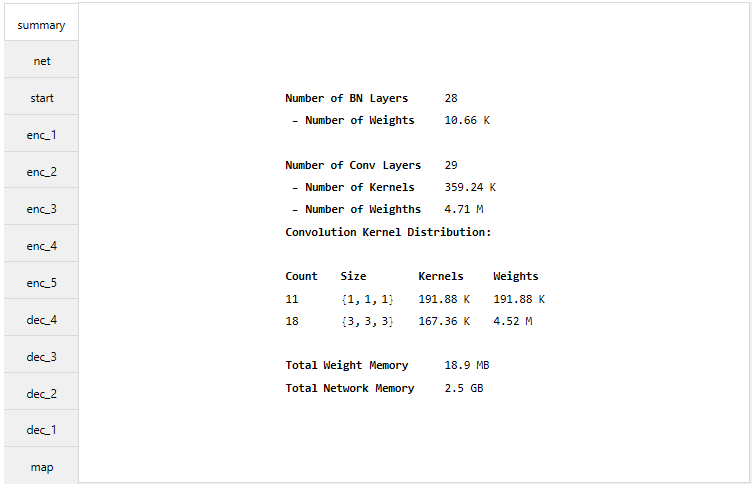
With the function MakeUnet a UNet is generated. The number of input channels, number of labels and the patch dimensions need to be given. With the fucntion NetSummary a summary of the network can be given.
net = MakeUnet[1, 15, {32, 112, 112}];
NetSummary[net, "Full"]
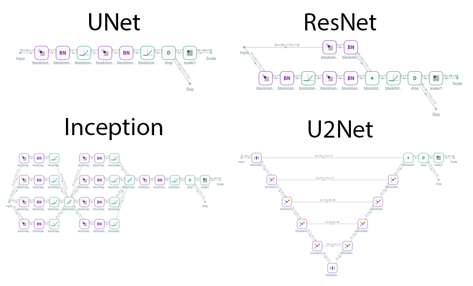
The UNet can be configured in various ways in both 2D and 3D in any depth needed. However for muscle segmentaion 3D is much better. Most common activation layers are availible and diffrent scaling and features per layer can be configured. The UNet architecture can be UNet, UNet+, or UNet++. The blocks used in the network can be a choise of:
- Convolution block
- Default UNet block
- ResNet block
- DenseNet block
- U2Net block
- Inception Block
Although there are many configureation options the recommendation is to use UNet architecture with ResNet blocks which is a right balance between reducing the weigths and having enough network complexity that still easily fits the memroy of most midrange GPUs for training.
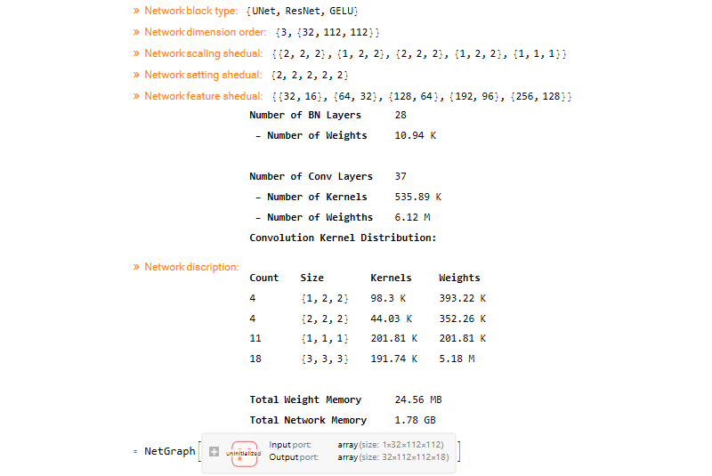
The configuration that is used for the networks provided with QMRITools is as given below.
MakeUnet[1, 18, {32, 112, 112},
  NetworkArchitecture -> "UNet", MonitorCalc -> True,
  DropoutRate -> 0.2, ActivationType -> "GELU", BlockType -> "ResNet",
  SettingSchedule -> Automatic,
  FeatureSchedule -> {32, 64, 128, 192, 320},
  DownsampleSchedule -> { {2, 2, 2}, {1, 2, 2}, {2, 2, 2}, {1, 2, 2}, {1, 1, 1} }]
4. Training Networks
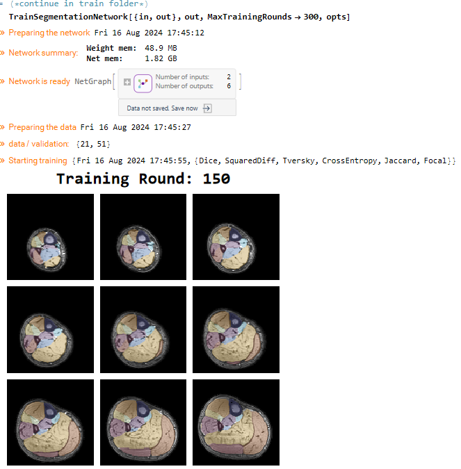
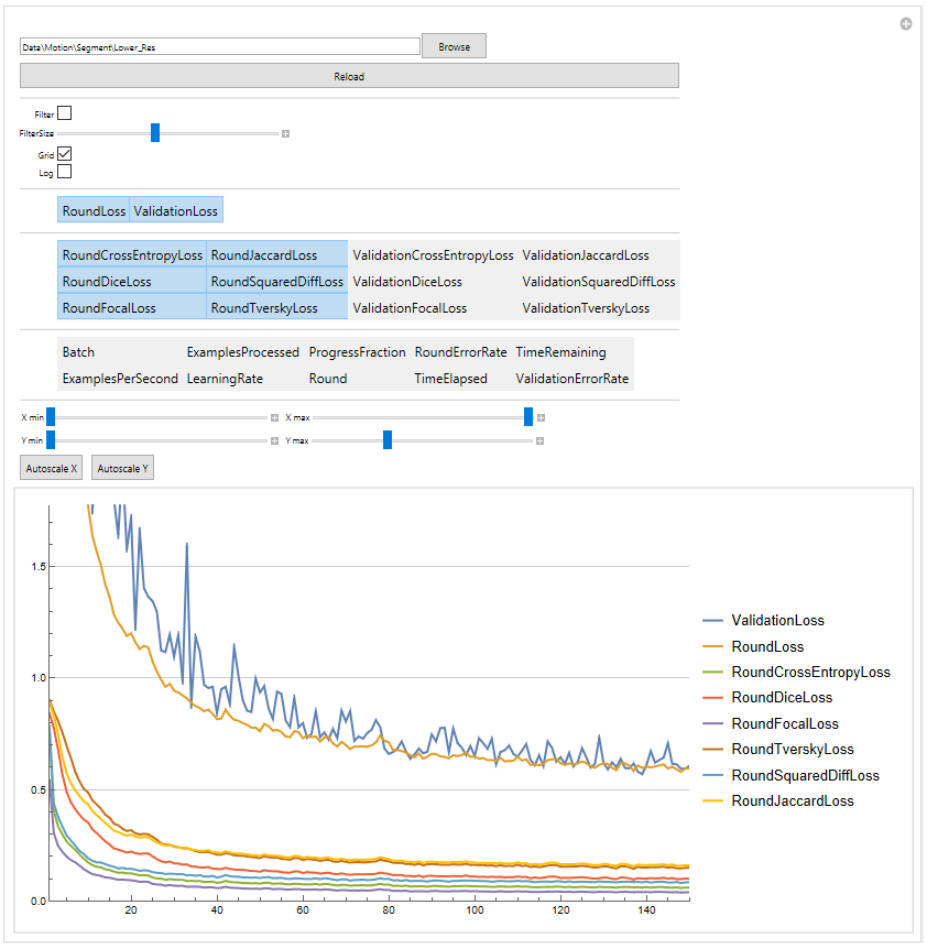
If all the data is prepared the training can begin. If the folder with the traindata is created with PrepareTrainData everything is set to go. With the following code the networks in QMRITools are trained. During the training a dynamic image of the training status is shown.
TrainSegmentationNetwork[{trainFolder, outputFolder},
  MaxTrainingRounds -> 150,
  LossFunction -> All,
  LearningRate -> 0.001, L2Regularization -> 0.0001,
  AugmentData -> True, DropoutRate -> 0.2,
  PatchSize -> {32, 112, 112}, PatchesPerSet -> 1,
  BatchSize -> 4, RoundLength -> 512,
  LoadTrainingData -> True, MonitorInterval -> 1,
  FeatureSchedule -> {32, 64, 128, 192, 320},
  DownsampleSchedule -> { {2, 2, 2}, {1, 2, 2}, {2, 2, 2}, {1, 2, 2}, {1, 1, 1} },
  BlockType -> "ResNet", NetworkArchitecture -> "UNet", ActivationType -> "GELU"
]
If the training is aborted by the user of for any other reason the trainig can be continues at any moment by specifying the outputFolder as a start position TrainSegmentationNetwork[{trainFolder, outputFolder}, outputFolder]. If no training has been performed but a pretrained network is availible this can also be used to start the training from TrainSegmentationNetwork[{trainFolder, outputFolder}, netFile].
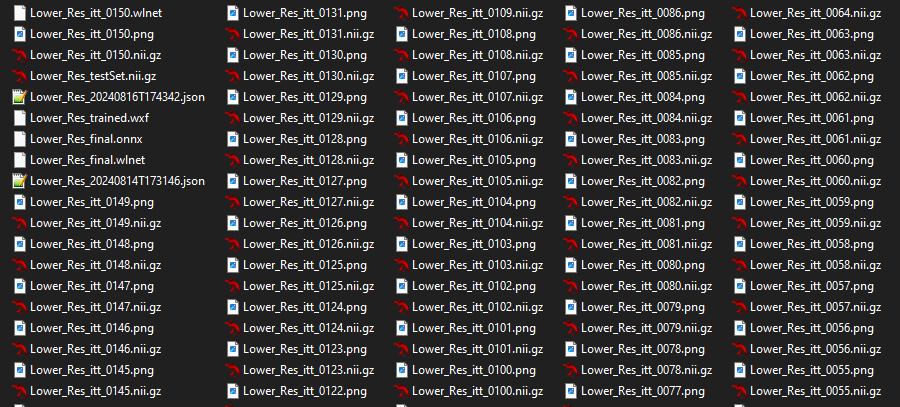
In the output folder all training progress is saved. When the training is initialized a test dataset will be made. For every itteration an progress image and segmentation data is made using this data. After each itteration the latest network is saved. If the training is completed a final network is also saved.
During the trainig the progress is saved in a logfile which can be veiwed with the ShowTrainLog function.
Since durint each training round the progress is saves as both images and segmentations stored as nifti files the framework allows to animate the training progress.
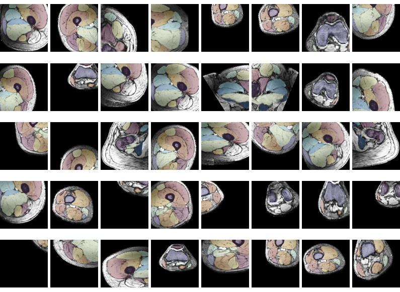
During the training the data is constantly augmented. The stored datasets are much larger than the patch used for training. Before a patch is selected from a random datasets the data is first augmentented. The augmentation is one of 7 possibilities, flip LR, rotate (LR, AP, FH), and scale (LR, AP, FH). Each of these happens with a chance of 50%. The location where the patch is selected is also seleceted random. Therefore, the network hardly ever sees the exact same patch twice. Below are 40 training patches all selected from the same dataset.
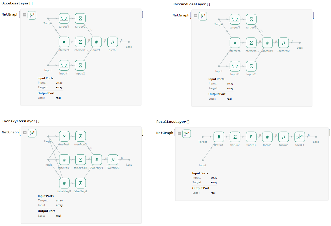
Next to the default loss layers availible in the Wolfram Language the toolbox also contains various loss functions dedicated to training segmentation networks. Available loss layers are DiceLossLayer, JaccardLossLayer, TverskyLossLayer, FocalLossLayer, MeanSquaredLossLayer and CrossEntropyLossLayer.
5. Using Networks
To use the integrated segemetation pipeline the function SegmentData should be used. However if custon networks are to be used the function ApplySegmentationNetwork is availible. For SegmentData a few custom scripts are implemented, which currently only are “Legs”, “LegBones” but more will be comming soon. For custom networks any network can be used with any data.
ApplySegmentationNetwork[data, network]
ApplySegmentationNetwork[{data1, data2, ...}, network]
ApplySegmentationNetwork[folder, network]
This will apply the segmentation network, which can be a NetGraph or a file name, to the given dataset list of datasets or all datasets in the folder.
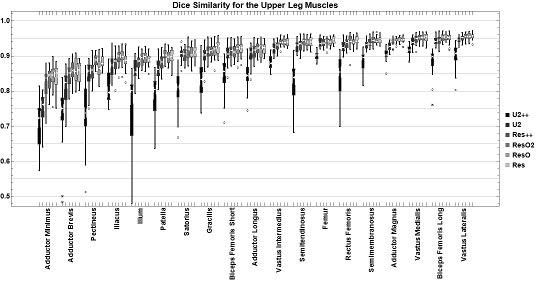
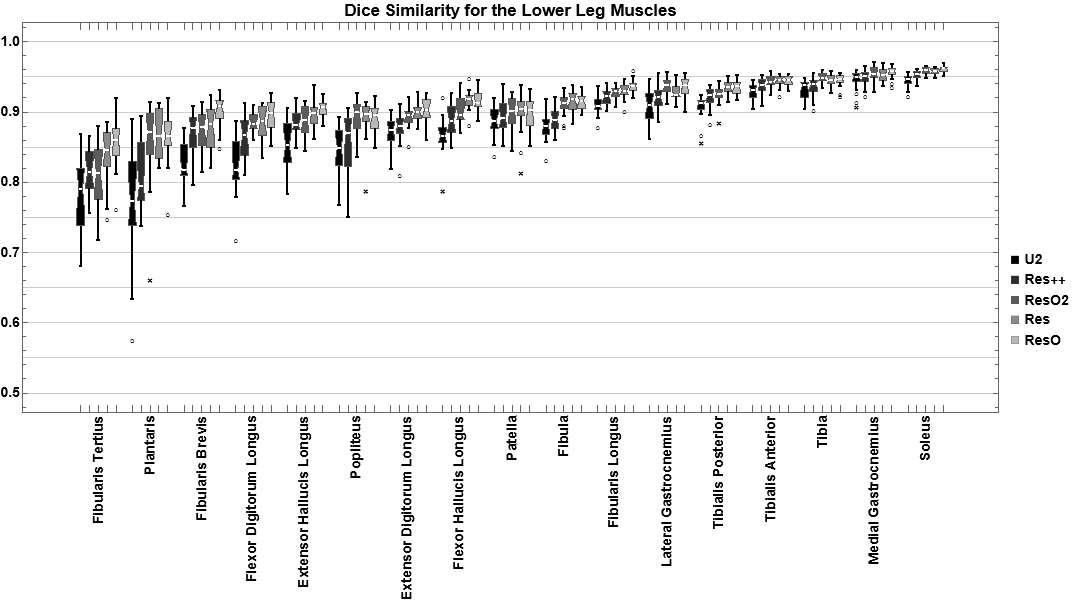
For the evaluation of segmentation networks multiple similarity mesasures have been implemented. The main ones are DiceSimilarity, JaccardSimilarity, and SufaceDistance. The latter can calcualte, amongst others, the mean, max, and 95% Hausdorff distance. During optimization of the networks in QMRITools multiple architectures have been tested. Below you can see the performance for the dice similarity metic for some architectures.

